Coupled Task Assignment for Hierarchical Multi-Agent Systems
A coupled task assignment framework for hierarchical multi-agent systems with applications to disaster response using aircraft and drone fleets.
Disclaimer: Some of the content in this report might be inaccurate or incorrect. Please refer to the paper version of this work for the most accurate information. The paper can be found here.
Motivation
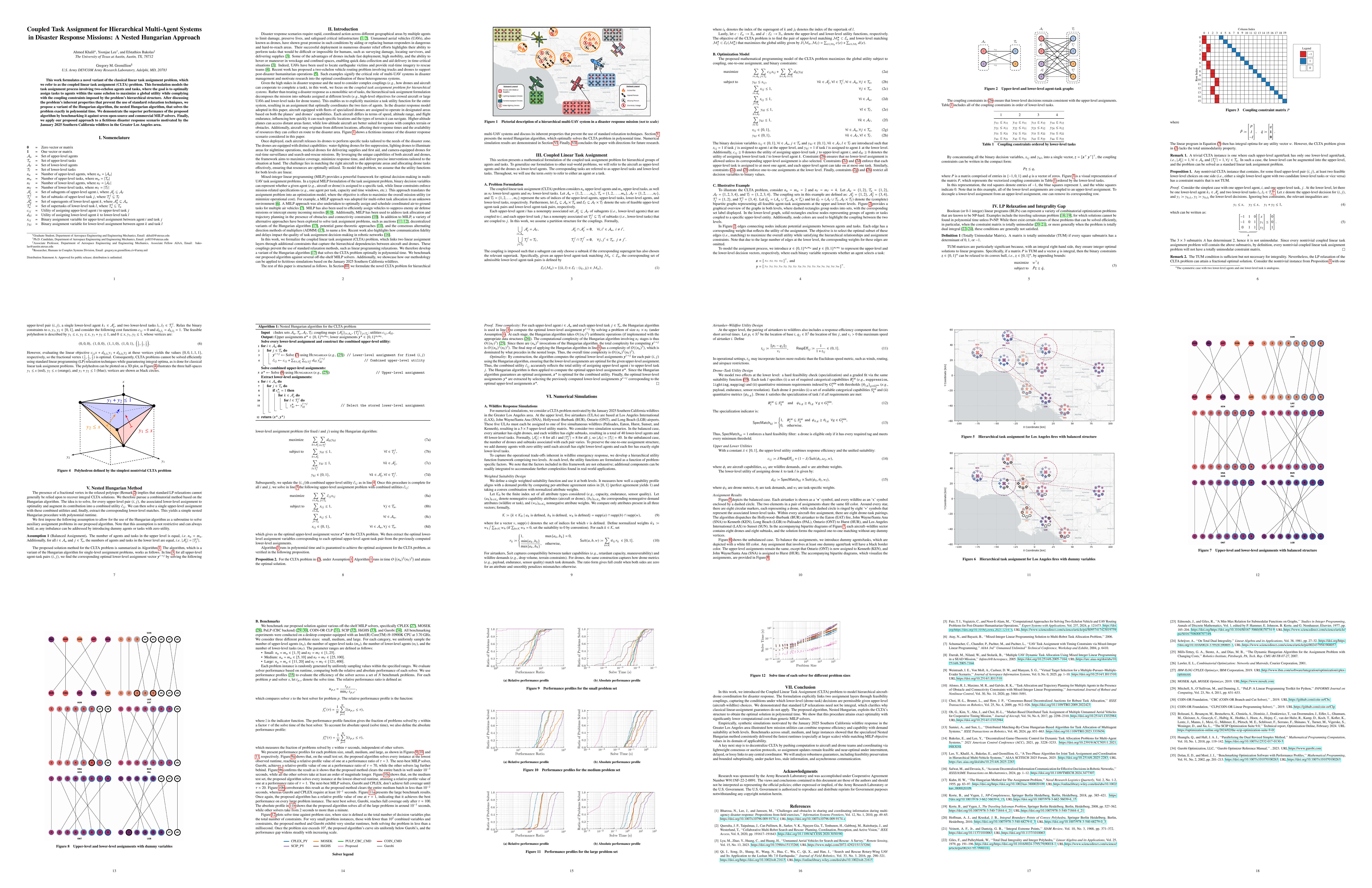
Efficient disaster response requires the deployment of multiple agents with varying capabilities to address tasks across different geographical areas. In this model, aircraft equipped with fleets of specialized drones are assigned to operate in designated areas based on both the planes’ and drones’ capabilities. Each aircraft differs in terms of speed, altitude range, and flight endurance, influencing how quickly it can reach specific locations and the types of terrain it can navigate. Higher-altitude planes can access distant areas faster, while low-altitude aircraft are better suited for regions with complex terrain or obstacles. Additionally, aircraft may originate from different locations, affecting their response times and the availability of resources they can collect en route to the disaster area.
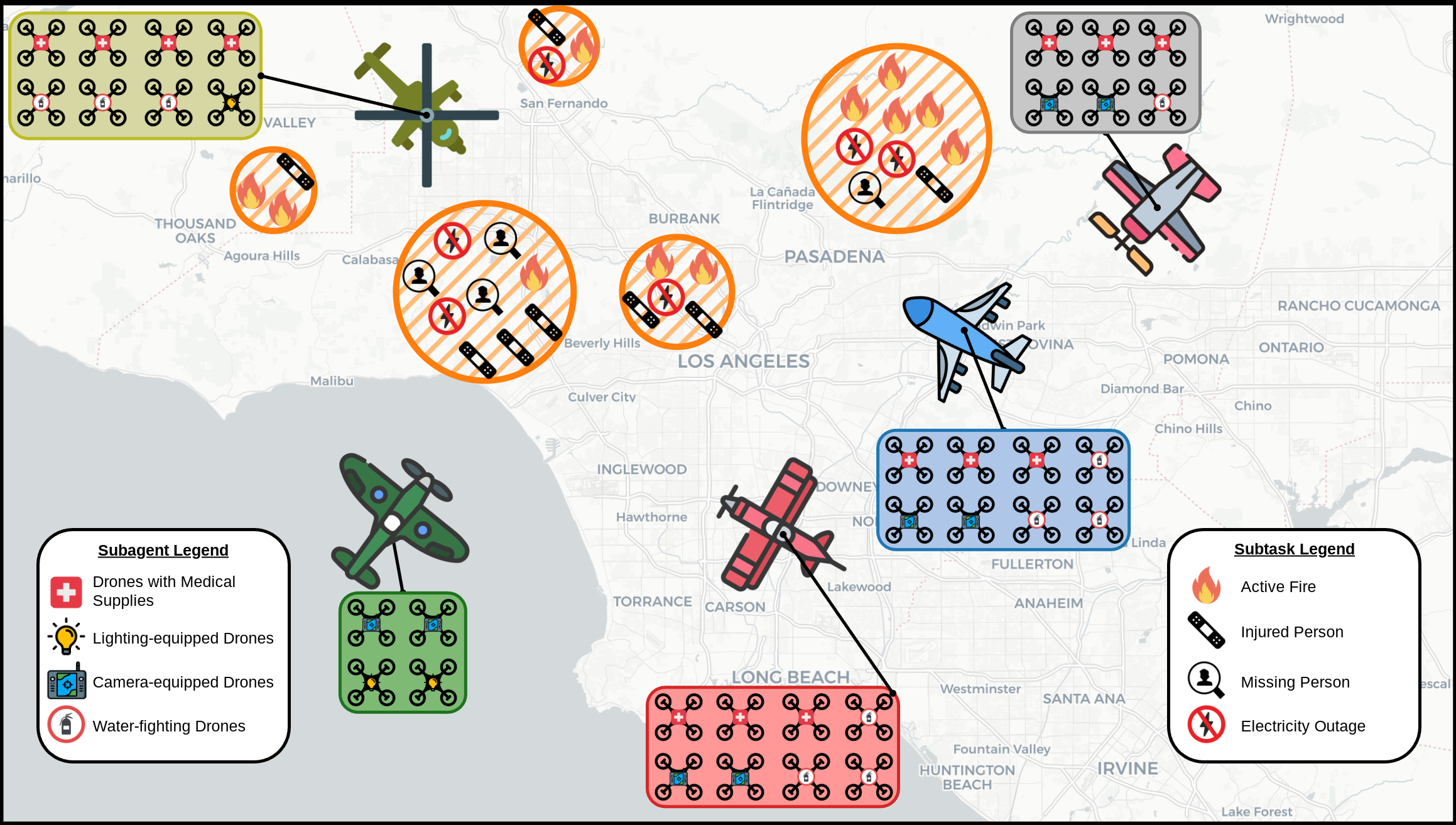
Once deployed, each aircraft releases its drones to perform specific tasks tailored to the needs of the disaster zone. The drones are equipped with distinct capabilities: water-fighting drones for fire suppression, lighting drones to illuminate areas for nighttime operations, medical drones for the delivery of supplies and first aid, and camera-equipped drones for real-time surveillance and search-and-rescue missions. By leveraging the unique capabilities of both aircraft and drones, the framework aims to maximize coverage, minimize response time, and deliver precise interventions tailored to the situation at hand. The challenge lies in matching the right aircraft to the appropriate areas and allocating drone tasks effectively, ensuring that resources are optimally utilized.
Problem Formulation
The Coupled Linear Task Assignment (CLTA) problem is a novel variant of the classical linear task assignment problem designed for hierarchical multi-agent systems. It models a two-echelon assignment process involving agents and tasks at different levels of a hierarchy.
Sets and Entities
Throughout this formulation, the term entity refers to either an agent or a task. The problem considers the following sets of indices:
- Upper-level agents (\(\mathcal{A}_{u}\)): \(\{1, 2, \dots, n_{u}\}\).
- Upper-level tasks (\(\mathcal{T}_{u}\)): \(\{1, 2, \dots, m_{u}\}\).
- Lower-level agents (\(\mathcal{A}_{l}\)): \(\{1, 2, \dots, n_{l}\}\).
- Lower-level tasks (\(\mathcal{T}_{l}\)): \(\{1, 2, \dots, m_{l}\}\).
Hierarchical Coupling
In this structure, a subagent can only choose a subtask if its corresponding superagent has also chosen the relevant supertask. This is defined by partition structures:
- \(\mathcal{A}_{l}^{i} \subseteq \mathcal{A}_{l}\) is the set of subagents (e.g., drones) coupled to upper-level agent \(i\) (e.g., aircraft).
- \(\mathcal{T}_{l}^{j} \subseteq \mathcal{T}_{l}\) is the set of subtasks coupled to upper-level task \(j\) (e.g., a specific wildfire zone).
These sets are assumed to be pairwise disjoint and nonempty, meaning each lower-level entity is coupled to exactly one upper-level entity.
Optimization Model
The goal of the CLTA problem is to find the pair of upper-level and lower-level matchings that maximize the global utility, representing the total effectiveness of the mission.
\[\begin{aligned} \text{maximize} \quad & \sum_{i \in \mathcal{A}_{u}} \sum_{j \in \mathcal{T}_{u}} c_{ij} x_{ij} + \sum_{k \in \mathcal{A}_{l}} \sum_{l \in \mathcal{T}_{l}} d_{kl} y_{kl} \\ \text{subject to} \quad & y_{kl} \le x_{ij}, && \forall k \in \mathcal{A}_{l}^{i}, \forall l \in \mathcal{T}_{l}^{j}, \forall i \in \mathcal{A}_{u}, \forall j \in \mathcal{T}_{u} \\ & \sum_{i \in \mathcal{A}_{u}} x_{ij} \le 1, && \forall j \in \mathcal{T}_{u} \\ & \sum_{j \in \mathcal{T}_{u}} x_{ij} \le 1, && \forall i \in \mathcal{A}_{u} \\ & \sum_{k \in \mathcal{A}_{l}} y_{kl} \le 1, && \forall l \in \mathcal{T}_{l} \\ & \sum_{l \in \mathcal{T}_{l}} y_{kl} \le 1, && \forall k \in \mathcal{A}_{l} \\ & x_{ij} \in \{0, 1\}, && \forall i \in \mathcal{A}_{u}, \forall j \in \mathcal{T}_{u} \\ & y_{kl} \in \{0, 1\}, && \forall k \in \mathcal{A}_{l}, \forall l \in \mathcal{T}_{l} \end{aligned}\]Constraint Breakdown
- Global Utility (Objective): Maximizes the combined utility of upper-level assignments (\(c_{ij}\)) and lower-level assignments (\(d_{kl}\)).
- Coupling Constraint (\(y_{kl} \le x_{ij}\)): Ensures that no lower-level assignment is allowed unless its corresponding upper-level assignment is also selected.
- One-to-One Matching: Constraints enforce that each task (at either level) is assigned to at most one agent, and each agent can take on at most one task.
- Binary Variables: Restricts all decision variables (\(x_{ij}\) and \(y_{kl}\)) to binary values (0 or 1), representing discrete assignment choices.
LP Relaxation and the Integrality Gap
Standard task assignment problems are often solved by relaxing binary constraints where decision variables must be exactly 0 or 1 into a continuous range [0, 1]. In many classical assignment problems, this linear program (LP) relaxation is guaranteed to yield integer solutions. However, the CLTA problem lacks this property. This means that generic solvers may produce “fractional” assignments such as assigning half of a drone to a task which are physically impossible to execute.
Illustrative Example of the Gap
To see why standard relaxation fails, consider a simple case with one upper-level agent-task pair $(i, j)$, a single lower-level agent $k_1$, and two potential lower-level tasks $l_1$ and $l_2$. When we relax the binary constraints, the core requirements are:
\[y_1 \le x, \quad y_2 \le x, \quad y_1 + y_2 \le 1\]If we assign a utility of zero to the aircraft assignment ($c_{ij} = 0$) and a utility of one to each drone task ($d_{k_1l_1} = d_{k_1l_2} = 1$), the objective function is:
\[\text{maximize} \quad 0 \cdot x + 1 \cdot y_1 + 1 \cdot y_2\]Evaluating the feasible polyhedron shows that the optimal solution occurs at a fractional vertex:
\[\text{Optimal fractional solution: } (x, y_1, y_2) = \left(\frac{1}{2}, \frac{1}{2}, \frac{1}{2}\right)\]In this fractional state, the solver gains a total utility of $1.0$. However, in a real-world mission, you cannot assign “half” an aircraft to enable “half” of two different drone tasks. Because the CLTA problem is not guaranteed to produce integer results through standard relaxation, specialized algorithms like the Nested Hungarian are required to find usable, optimal solutions.
Visualization of the Feasible Polyhedron
The 3D plot below visualizes the feasible region for this example. The three colored planes represent the half-spaces $y_1 \le x$ (red), $y_2 \le x$ (orange), and $y_1 + y_2 \le 1$ (blue).
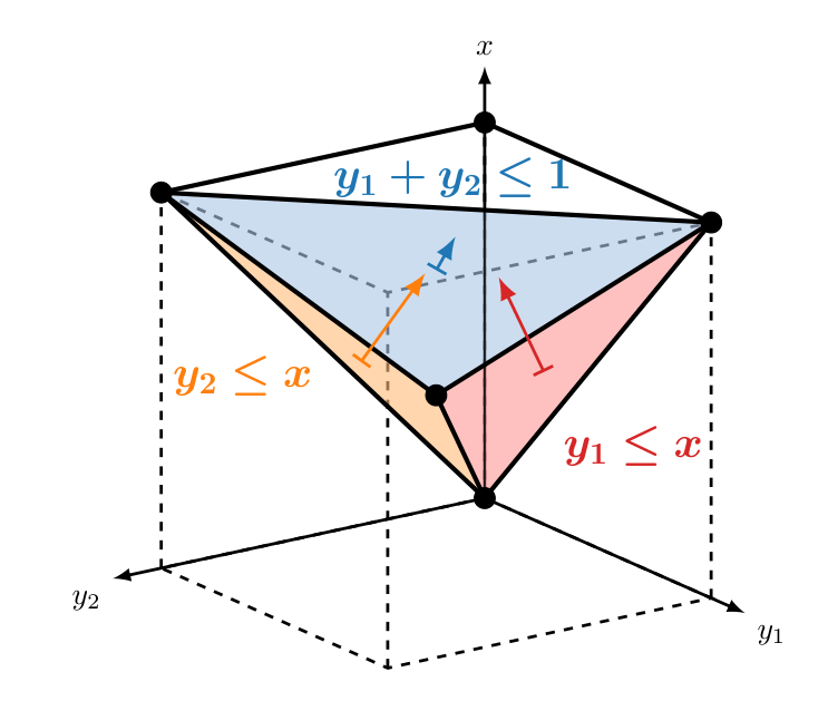
The black circles highlight the vertices of the polyhedron, including the fractional vertex $(0.5, 0.5, 0.5)$.
Nested Hungarian Method
Standard LP relaxations cannot be relied upon to recover integral solutions for the CLTA problem because of the fractional vertices in the relaxed polytope. To solve this exactly in polynomial time, we use a combinatorial approach called the Nested Hungarian Method. The core idea is to solve the optimal lower-level assignment for every possible upper-level pair and then use those results to inform the final upper-level decision.
The Algorithm
The algorithm follows a three-stage nested process to find the global optimum.
1. Precompute Lower-Level Utilities
For every possible upper-level agent-task pair $(i, j)$, we solve a local lower-level assignment problem. This identifies the best drone-to-task matching that would happen if that specific aircraft was assigned to that specific fire.
\[\text{maximize} \quad \sum_{k \in \mathcal{A}_{l}^{i}} \sum_{l \in \mathcal{T}_{l}^{j}} d_{kl} y_{kl}\]2. Construct Combined Upper-Level Utilities
We then create a “combined” utility, \(\hat{c}_{ij}\), for each aircraft-wildfire pair. This value includes the aircraft’s own utility ($c_{ij}$) plus the total utility from its optimal fleet of drones precomputed in Step 1:
\[\hat{c}_{ij} \leftarrow c_{ij} + \sum_{k \in \mathcal{A}_{l}^{i}} \sum_{l \in \mathcal{T}_{l}^{j}} d_{kl} y_{kl}^{i \rightarrow j}\]3. Solve Final Assignments
Finally, we solve a standard single-level assignment problem at the upper level using these combined utilities:
\[\text{maximize} \quad \sum_{i \in \mathcal{A}_{u}} \sum_{j \in \mathcal{T}_{u}} \hat{c}_{ij} x_{ij}\]Once the optimal aircraft assignments ($x^\star$) are found, we simply extract the corresponding precomputed drone assignments ($y^\star$) to complete the mission plan.
Complexity and Scalability
Despite the “nested” nature of the problem, this algorithm is remarkably efficient and runs in polynomial time.
- Runtime Complexity: The overall time complexity is \(O((n_{u})^{2}(n_{l})^{3})\).
- Performance: Since it targets the specific structure of the CLTA problem, it reaches exact optimality significantly faster than generic MILP solvers, which must navigate complex branching and relaxation steps.
Numerical Simulations
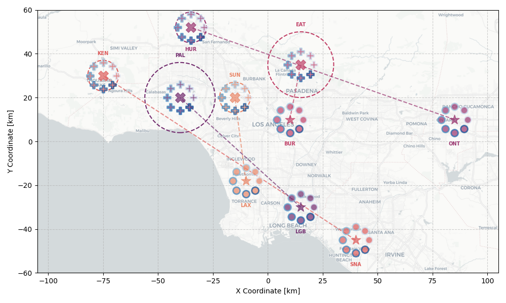
Wildfire Response Simulations
The CLTA problem is evaluated through a simulation motivated by the January 2025 Southern California wildfires in the Greater Los Angeles area. The scenario features five airtankers (upper-level agents) based at major airports: LAX, SNA, BUR, ONT, and LGB. These tankers are assigned to five simultaneous wildfires: Palisades, Eaton, Hurst, Sunset, and Kenneth.
Two scenarios are considered:
- Balanced case: Each tanker has eight drones and each fire has eight subtasks, totaling 40 lower-level agents and 40 tasks.
- Unbalanced case: The number of drones and subtasks varies; dummy agents with zero utility are added to maintain the one-to-one assignment structure.
Weighted Suitability Design
A weighted suitability function measures how well a capability profile aligns with a demand profile. Attributes such as capacity, endurance, and sensor quality are compared using normalized weights.
The set of comparable attributes is defined as:
\[\mathcal{K} \coloneqq \{k\in \mathcal{K}_0 \mid a_k\ \text{is defined},\ b_k\ \text{is defined},\ w_k\ \text{is defined}\}\]The suitability is computed as:
\[r_k \coloneqq \begin{cases} 1, & \max\{a_k,b_k\}=0, \\ \frac{\min\{a_k,b_k\}}{\max\{a_k,b_k\}}, & \text{otherwise}, \end{cases} \qquad \textsf{Suit}(a,b,w) \coloneqq \sum_{k\in \mathcal{K}} \tilde w_k\, r_k \ \in [0,1]\]Airtanker–Wildfire Utility Design
Upper-level utility includes a response-efficiency component favoring short arrival times. Using aircraft speed ($v_i$), base location ($p_i$), and fire location ($q_j$), efficiency is defined as:
\[t_{ij} \coloneqq \frac{\|p_i-q_j\|_2}{v_i}, \qquad \textsf{RespEff}_{ij} \coloneqq \frac{1}{1+t_{ij}} \in (0,1]\]Drone–Task Utility Design
Lower-level drones must pass a hard feasibility check (specialization) before a graded fit is calculated. A drone matches a task if it meets all categorical requirements and quantitative minimums.
The specialization indicator is defined as:
\[\textsf{SpecMatch}_{k l} \coloneqq \begin{cases} 1, & R_{l}^{\text{cat}} \subseteq S_k^{\text{cat}}\ \ \text{and}\ \ \psi_{k,g} \ge \theta_{l,g}\ \ \forall g\in G_{l}^{\min}, \\ 0, & \text{otherwise}. \end{cases}\]Upper and Lower Utilities
Combining response efficiency and suitability with a weight factor $\lambda \in [0,1]$, the final utilities are:
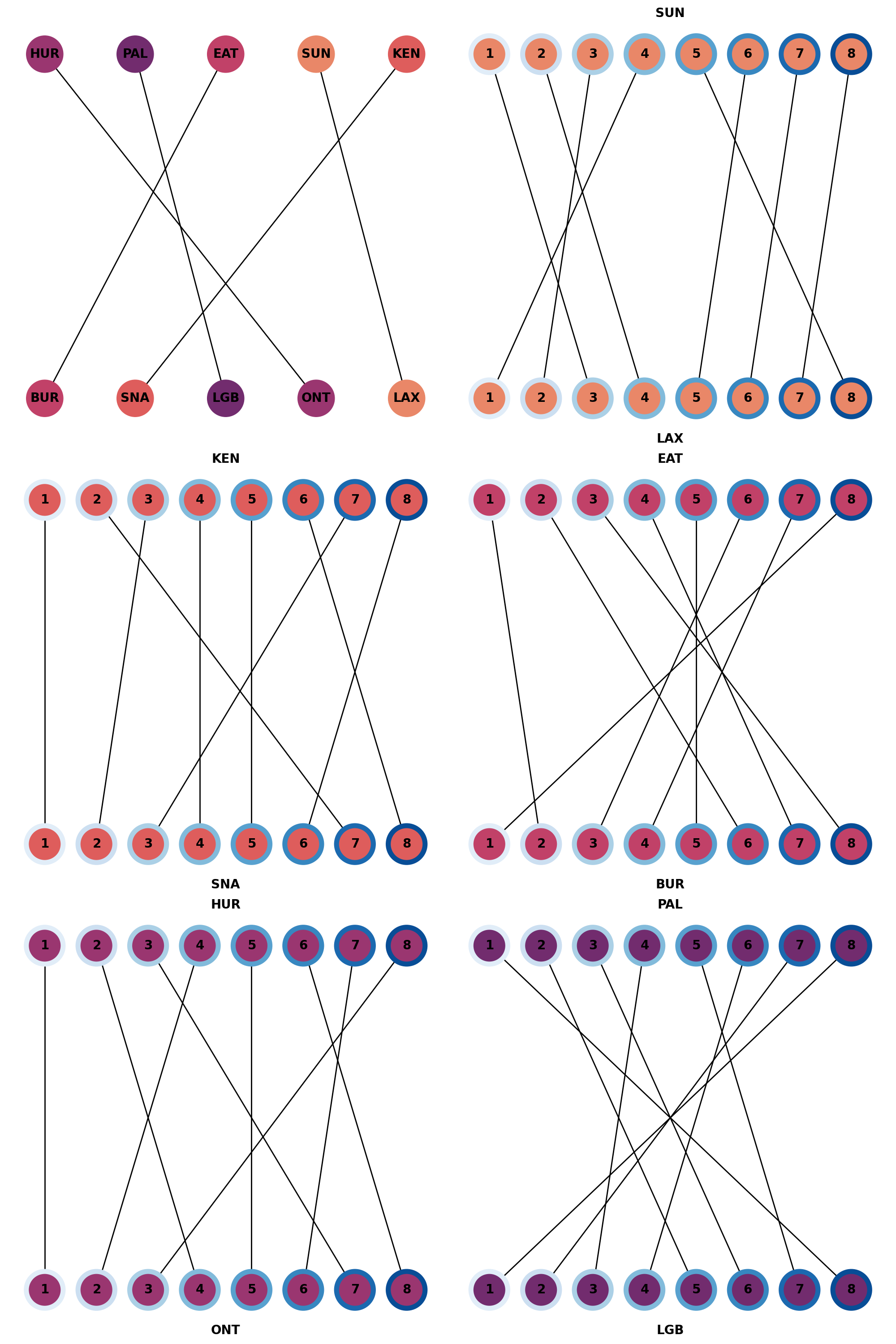
\[c_{ij} \coloneqq \lambda \, \textsf{RespEff}_{ij} + (1-\lambda) \, \textsf{Suit}(\phi_i,\omega_j,w)\] \[d_{k l} \coloneqq \textsf{SpecMatch}_{k l} \times \textsf{Suit}(\psi_k,\theta_l,w_l)\]Assignment Results
The algorithm effectively dispatches aircraft and coordinates drone fleets. In the balanced case, the BUR tanker is assigned to Eaton, SNA to Kenneth, LGB to Palisades, ONT to Hurst, and LAX to Sunset.
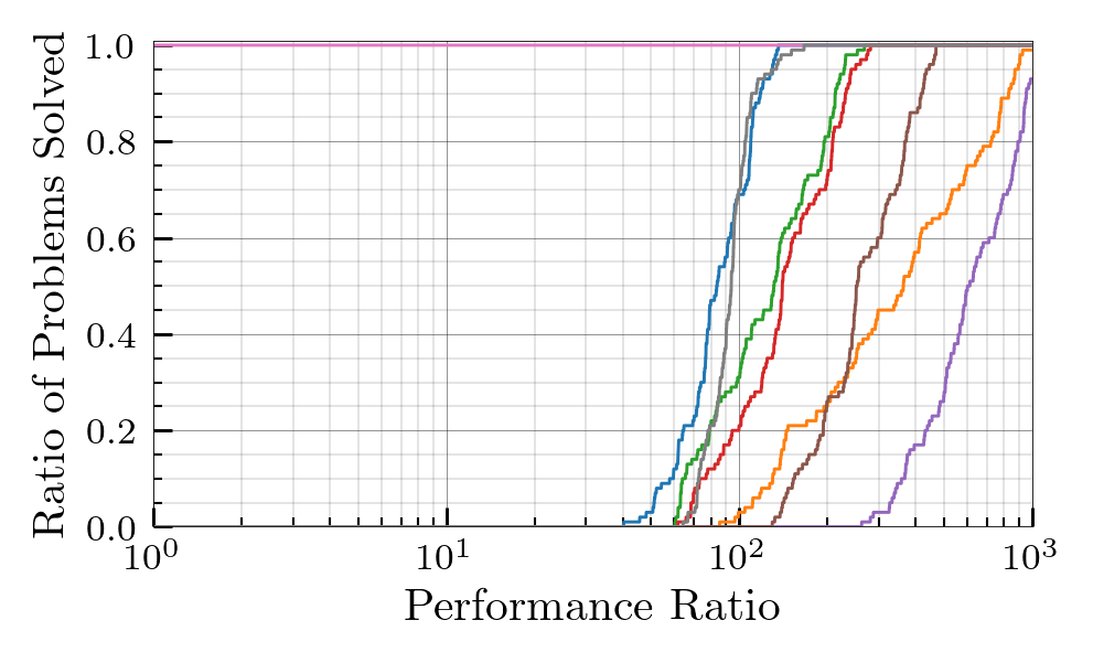
Benchmarks
The Nested Hungarian algorithm was benchmarked against seven major MILP solvers, including Gurobi and CPLEX. Problems were categorized as Small ($n_l \in [1,25]$), Medium ($n_l \in [25,100]$), and Large ($n_l \in [121,400]$).
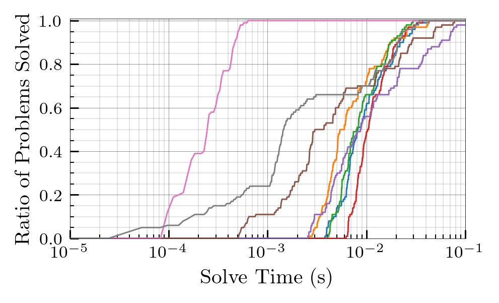
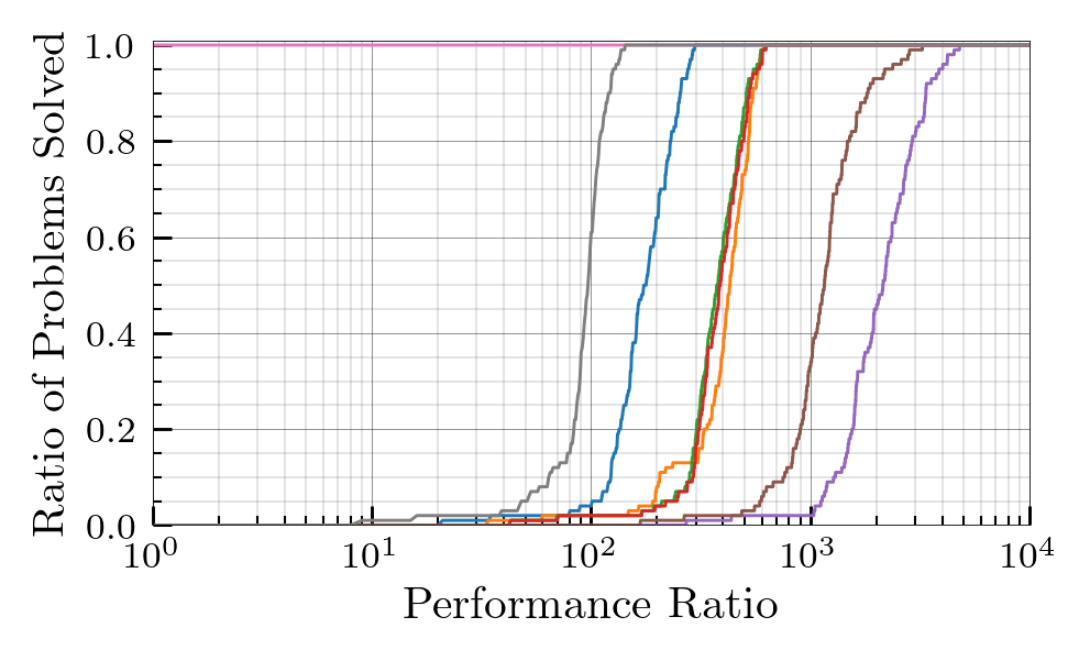
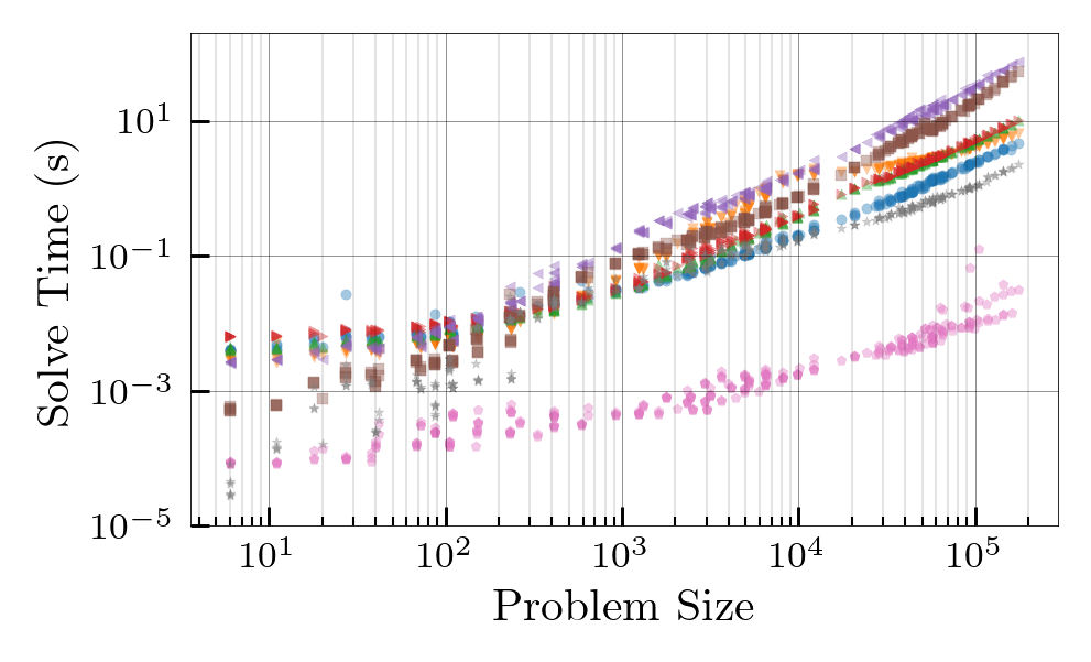
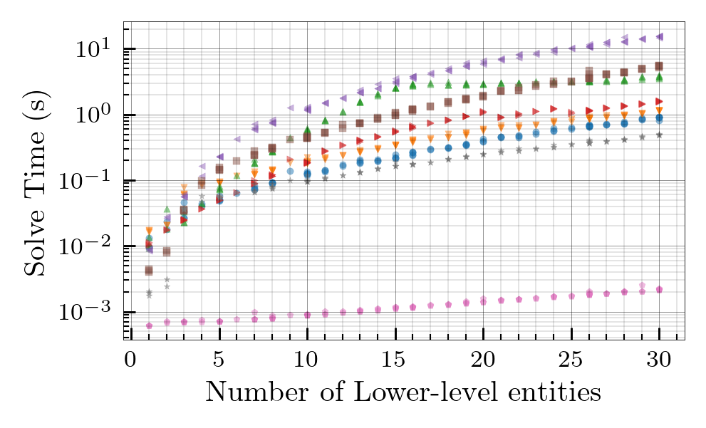
- Performance Profiles: The proposed algorithm achieved the best observed runtime on every instance in the Large test set, clearing them in roughly $10^{-1}$ seconds.
- Efficiency Gap: For problems with over $10^2$ variables and constraints, the Nested Hungarian method uniformly outperforms Gurobi, with the performance gap widening steadily as the scale increases.
Small Set Performance Profile Results
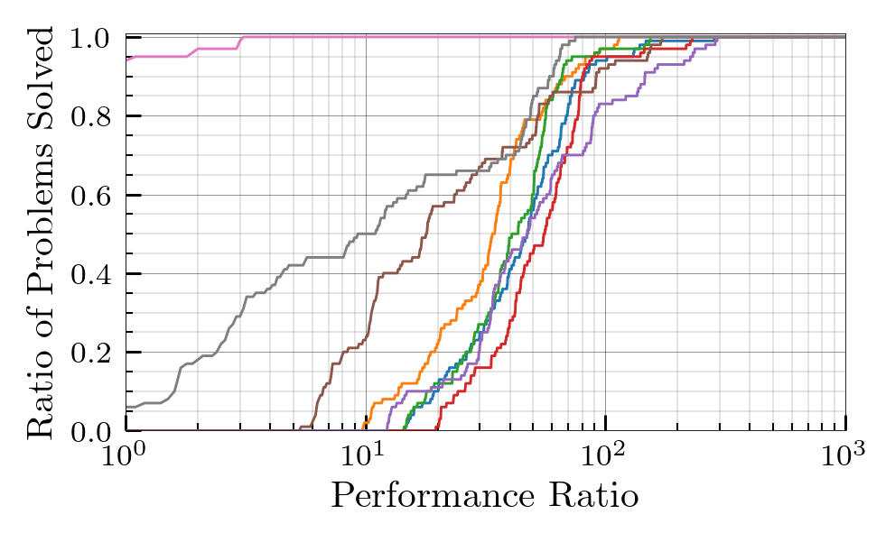
Medium Set Performance Profile Results
Large Set Performance Profile Results
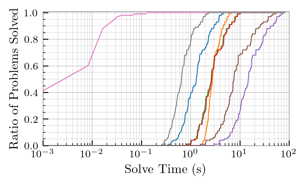
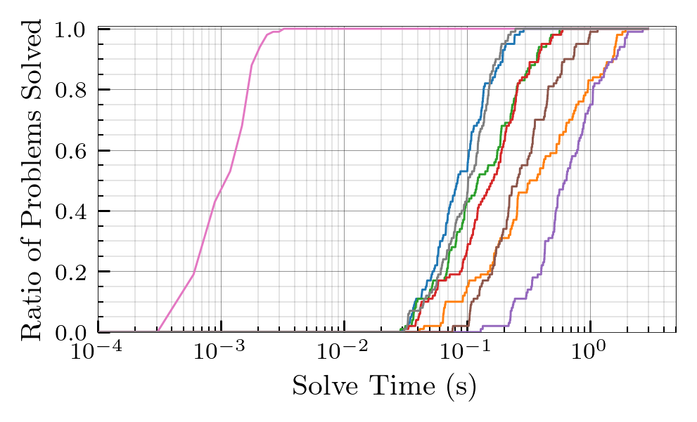
Solve Time Analysis
Miscellaneous CLTA as a Binary Linear Program
The CLTA problem can be formulated as a binary linear program (BLP):
\[\begin{split} &{\text{minimize}} \quad&& c^\top z \\ & \text{subject to} && A z \preceq b \\ &&& z_i \in \{0,1\}, \quad i = 1, \ldots, N. \end{split} \tag{BLP}\]Note that for the time being, we revert back to the binary constraints.
The boolean linear program is known to be NP-hard and was included as one of Karp’s 21 NP-complete problems
Motivated by the coupled linear task assignment problem, the work below has some half-baked methods of “solving” the generalized BLP.
Difference of Convex Programming
The BLP is a subclass of difference of convex (DC) programming problems
While global solutions of DC problems can be found using branch-and-bound
Relaxation Methods for BLPs
Here, we discuss two relaxation methods for solving BLPs: the linear program relaxation (LP) and the Lagrangian relaxation (LR)
Linear Program Relaxation (LP)
By replacing the integrality constraint with the box constraint, \(0\le z_i \le 1\), the BLP becomes the following primal form of the linear program relaxation (LP):
\[\begin{equation} \begin{aligned} \label{eqn4:LPRelaxation} &{\text{minimize}} && c^\top z \\ & \text{subject to} && A z \preceq b \\ &&& 0 \le z_i \le 1, \quad i = 1, \ldots, N. \end{aligned} \tag{LP-P} \end{equation}\]The Lagrangian, \(L\), is given by
\[\begin{align} L(z, u, v, w) &= c^\top z + u^\top (Az -b) -v^\top z + w^\top (z- \ones) \\ &= (c+ A^\top u - v +w)^\top z - u^\top b - w^\top \ones. \end{align}\]The corresponding Lagrange dual function, \(g\), is given by
\[\begin{align} g(u, v, w) &= \inf_{z} \left[ (c+ A^\top u - v +w)^\top z - u^\top b - w^\top \ones \right]\\ &= - u^\top b - w^\top \ones + \inf_{z} \left[ (c+ A^\top u - v +w)^\top z \right]. \end{align}\]Therefore,
\[\begin{equation} g(u, v, w)= \begin{cases} - u^\top b - w^\top \ones & \text{if } c+ A^\top u - v +w = 0 \\ -\infty & \text{otherwise}. \end{cases} \end{equation}\]The dual problem is then given by,
\[\begin{equation} \begin{aligned} \label{eqn5:LPRelaxationDual} &{\text{maximize}} && - u^\top b - w^\top \ones \\ & \text{subject to} && c+ A^\top u - v +w = 0 \\ &&& u \succeq 0, v \succeq 0, w \succeq 0. \end{aligned} \tag{LP-D} \end{equation}\]Lagrangian Relaxation (LR)
By replacing the integrality constraint with the concave quadratic constraint, \(z_i (1 - z_i) =0\), the BLP becomes,
\[\begin{equation} \begin{aligned} \label{eqn5:LagrangianRelaxation} &{\text{minimize}} && c^\top z \\ & \text{subject to} && A z \preceq b \\ &&& z_i (1 -z_i) =0, \quad i = 1, \ldots, N. \end{aligned} \tag{LR-P} \end{equation}\]The Lagrangian, \(L\), is given by
\[\begin{align} L(z, \mu, \nu) &= c^\top z + \mu^\top (Az -b) -\nu^\top z + z^\top \diag(\nu) z \\ &= -\mu^\top b + \left(c+ A^\top \mu - \nu \right)^\top z + z^\top \diag(\nu)z. \end{align}\]The corresponding Lagrange dual function, \(g\), is given by
\[\begin{align} g(\mu, \nu) &= \inf_{z} \left[ c^\top z + \mu^\top (Az -b) - \nu^\top z + z^\top \diag(\nu) z \right]\\ &= -\mu^\top b + \inf_{z} \left[\left(c+ A^\top \mu - \nu \right)^\top z + z^\top \diag(\nu)z \right]. \end{align}\]The function inside the infimum is quadratic in \(z\) and is separable across components due to the diagonal structure \(\diag(\nu)\). For each \(i\), when \(\nu_i > 0\), the function \(f_i (z_i) = \nu_i z_i^2 + ( c_i + a_i^\top \mu - \nu_i) z_i\) is convex in \(z_i\), where \(a_i\) is the \(i\)th column of \(A\). Using the first-order necessary conditions for optimality,
\[\begin{align} \nabla_{z_{i}} f_i (z_i) &= 2 \nu_i z_i + c_i + a_{i}^{\top} \mu - \nu_i = 0, \end{align}\]the optimal value occurs at
\[\begin{align} z_{i}^\star = - \frac{c_i + a_i^\top \mu - \nu_i}{2 \nu_i}. \end{align}\]The value at this point is
\[\begin{align} f_i (z_{i}^\star) &= \nu_i \left[\frac{-(c_i + a_i^\top \mu - \nu_i)}{2 \nu_i} \right]^2 - (c_i + a_i^\top \mu - \nu_i) \frac{-(c_i + a_i^\top \mu - \nu_i)}{2 \nu_i} \\ &= \frac{-(c_i + a_i^\top \mu - \nu_i)^2}{4 \nu_i}. \end{align}\]When \(\nu_i = 0\), the function is linear. Thus, if \(c_i + a_i^\top \mu \ge 0\), then it has an infimum of \(0\). If \(c_i + a_i^\top \mu < 0\), then it has an infimum of \(- \infty\).
Therefore,
\[\begin{equation} g(\mu, \nu)= \begin{cases} -b^\top \mu - \frac{1}{4} \sum_{i=1}^N \frac{(c_i+ a_i^\top \mu - \nu_i)^2}{\nu_i} & \text{if } \nu \succeq 0\\ -\infty & \text{otherwise.} \end{cases} \end{equation}\]The resulting dual problem is then given by,
\[\begin{equation} \begin{aligned} & {\text{maximize}} && -b^\top \mu - \frac{1}{4} \sum_{i=1}^N \frac{(c_i+ a_i^\top \mu - \nu_i)^2}{\nu_i} \\ & \text{subject to} && \nu \succeq 0. \end{aligned} \end{equation}\]The second term can be simplified by finding its supremum. Let \(k_i \coloneqq c_i + a_i^\top \mu\). To find the supremum value of
\[\begin{align} \phi(\nu_i) = - \frac{(k_i - \nu_i)^2}{\nu_i}, \end{align}\]compute the derivative using the quotient rule:
\[\begin{align} \nabla_{v_{i}} \phi (v_i) &= -\frac{-2(k_i - \nu_i) \nu_i - (k_i \nu_i)^2}{\nu_i^2} \\ &= \frac{k_i^2 - \nu_i^2}{\nu_i^2}. \end{align}\]Using the first-order necessary conditions of optimality,
\[\begin{align} \nabla_{v_{i}} \phi (v_i) = 0 \implies k_i^2 - \nu_i^2 = 0 \implies \nu_i = |k_i|. \end{align}\]If \(k_i \le 0\), we have that \(\nu_i = -k_i\), thus,
\[\begin{align} \phi (\nu_i) &= \frac{(k_i - (- k_i))^2}{k_i^2} = 4 k_i \\ &= 4 (c_i + a_i^\top \mu). \end{align}\]If \(k_i \ge 0\), we have that \(\nu_i = k_i\), thus,
\[\begin{align} \phi (\nu_i) &= \frac{(k_i - k_i)^2}{k_i^2} \\ &= 0. \end{align}\]The second term can thus be simplified to
\[\begin{equation} \begin{aligned} \sup_{\nu_i \ge 0} \left(- \frac{(c_i +a_i^\top \mu -\nu_i)^2}{\nu_i} \right) &= \begin{cases} 4(c_i + a_i^\top \mu), & c_i + a_i^\top \mu \le 0\\ 0, & c_i + a_i^\top \mu \ge 0 \end{cases} \\ &= 4 \min \{0, (c_i +a_i^\top \mu)\}. \end{aligned} \end{equation}\]Thus, the dual problem is given by,
\[\begin{equation} \begin{aligned} & {\text{maximize}} && -b^\top \mu + \sum_{i=1}^{N} \min \{0, c_i +a_i^\top \mu \}\\ & \text{subject to} && \mu \succeq 0. \end{aligned} \tag{LR-D} \end{equation}\]This is equivalent to the dual problem of the LP relaxation given by LP-D, so both problems give the same lower bound. This relationship between optimal objective values can be summarized as,
\[\text{BLP} = \text{LR-P} \ge \text{LR-D} = \text{LP-D} = \text{LP-P}.\]This natural relation lays the foundation for the wide adoption of LP relaxations in solving integer linear programs
Augmented Lagrangian Relaxation (ALR)
Taking inspiration from both relaxations, the following augmented Lagrangian formulation is introduced. The following combines both methods by defining the optimization domain as the interval \([0,1]\) and by using the concave quadratic function as a penalty function. The Lagrangian, \(L\), is given by
\[\begin{align} % L (z, \mu; \rho, \gamma) &= c^\top z + \mu^\top \max\{0, Az -b\} + \frac{\rho}{2} \left[\ones^\top \max\{0, Az -b\}^2\right] +\frac{\gamma}{2} \left[ z^\top (\ones-z) \right],\\ L(z, \mu, \nu; \rho, \gamma) &= c^\top z + \mu^\top \max\{0, Az -b\} + \frac{\rho}{2} \left[ \ones^\top \max\{0, Az -b\}^2 \right] +\frac{\gamma}{2} \left[ \nu^\top z - z^\top \diag(\nu) z \right]. \end{align}\]where \(\mu \in \mbf{R}^m\) is the vector of Lagrange multipliers and \(\rho, \gamma \in \mbf{R}_+\) are penalty parameters such that \(\rho > \gamma\). Notice that the first three terms are convex, while the last is concave quadratic. Additionally, \(\nabla_z L\), is given by
\[\begin{align} \nabla_z L (z, \mu; \rho, \gamma) &= c + A^\top \mu + A^\top I_{\rho} (A z -b) +\frac{\gamma}{2} (\ones - 2z), \end{align}\]where \(I_\rho\) is a diagonal matrix defined as
\[\begin{equation} I_{\rho, ii} = \begin{cases} \rho & \text{if } (A z - b)_i > 0 \lor \mu_i > 0, \\ 0 & \text{otherwise}. \end{cases} \end{equation}\]The equivalence of the BLP and the problem of minimizing a concave quadratic objective function over a convex set is well-known
Semi-Definite Programming (SDP) Relaxation
Relaxing the binary constraint \(w \in \{-1,1\}^n\) to \(w^\top w = n\), where \(n\) is the number of decision variables, the BLP can be formulated as the following optimization problem:
\[\begin{equation} \begin{aligned} \label{eqn:} &{\text{minimize}} && c^\top w \\ & \text{subject to} && A w \preceq d \\ &&& w^\top w = n, \end{aligned} \end{equation}\]where \(d = 2b - A \ones\). The Lagrangian, \(L\), is given by
\[L = c^\top w + \mu^\top \max \{0, (A w - d)\}^2 + \nu (w^\top w - n).\]Note that the first constraint is being squared. Is this tight to the BLP?
Let’s consider the following simple problem, where \(a \in \mbf{R}^n\) and \(t \in \mbf{R}\):
\[\begin{equation} \begin{aligned} &\minimize \limits_{x} && c^\top x \\ & \text{subject to} && a^\top x = t, \\ &&& x \in \{-1,1\}^n. \end{aligned} \end{equation}\]We first replace the binary constraint with the equivalent rank-one constraint \(x^\top x = n\). However, this constraint is non-convex and is therefore relaxed to the following set of convex constraints:
\[\begin{equation} \Tr(X) = n, \quad X \succeq x x^\top \iff \begin{pmatrix} X & x \\ x^\top & 1 \end{pmatrix} \succeq 0. \end{equation}\]The resulting optimization problem is then given by
\[\begin{equation} \begin{aligned} \label{eqn:SDP} &\minimize \limits_{X, x} && c^\top x \\ & \text{subject to} && \begin{pmatrix} X & x \\ x^\top & 1 \end{pmatrix} \succeq 0, \\ &&& \Tr({X}) = n, \\ &&& a^\top x = t, \end{aligned} \tag{SDP} \end{equation}\]which is equivalent to the following problem with the linear constraint squared \((a^\top x - t)^2 = 0\), resulting in the following problem:
\[\begin{equation} \begin{aligned} &\minimize \limits_{X, x} && c^\top x \\ & \text{subject to} && \begin{pmatrix} X & x \\ x^\top & 1 \end{pmatrix} \succeq 0, \\ &&& \Tr(X) = n, \\ &&& \Tr(a a^\top X) - 2 t a^\top x + t^2 = 0. \end{aligned} \end{equation}\]Given the PSD constraint and the fact that
\[\begin{equation} \Tr(a a^\top X) - 2 t a^\top x + t^2 = \Tr\left(\begin{pmatrix} X & x \\ x^\top & 1 \end{pmatrix} \begin{pmatrix} a a^\top & -t a \\ -t a^\top & t^2 \end{pmatrix} \right), \end{equation}\]the squared linear constraint implies that
\[\begin{equation} \begin{pmatrix} X & x \\ x^\top & 1 \end{pmatrix} \begin{pmatrix} a \\ -t \end{pmatrix} = 0, \end{equation}\]which is equivalent to \(X a = t x\) and \(a^\top x = t\). This is equivalent to a projection of the problem into a space of dimension \(n-1\).